Example of an state observer to estimate the perturbed component of the body weight trajectory

Case study 3. Known theoretical trajectory.

In this example, we show the use of state observers to quantify dynamic perturbations. An observer is an object that combines a mathematical model and on-line data to estimate unmeasured variables

 knitr::opts_chunk$set(message = FALSE)

library("deSolve")
library(ggplot2)
library(ggExtra)
library(gridExtra)

# Loading the measured noisy data [time (d) animal body weight (kg)]
ynoise  <- read.table("ynoise.txt");
DN  <- data.frame(ynoise);
colnames(DN)<- c("time","BW");
tN <- DN$time
yN <- DN$BW

# Loading the measured filtered data [time (d) animal body weight (kg)]
ysmooth <- read.table("ysmooth.txt");
DS  <- data.frame(ysmooth);
colnames(DS)<- c("time","BW");
tS <- DS$time
yS <- DS$BW

# Loading the perturbation factor used to generate the simulated data 

perturbfactor<- read.table("perturbfactor.txt");
DP  <- data.frame(perturbfactor);
colnames(DP)<- c("time","Fi");
tP <- DP$time
yP <- DP$Fi

 # Dynamic model
tspan=tS; 

dy<- function(t, state,parameters) {  #ODE function observer
  with(as.list(c(state,parameters)), {
    
    # model parameters 
    # p1 = 0.05
    # p2 = 0.02
    
    # observer parameters
    #w1 =  4.0
    #w2 =  0.5
    
    #ysmooth <- read.table("ysmooth.txt");
    #DS  <- data.frame(ysmooth);
    #colnames(DS)<- c("time","BW");
    #tS <- DS$time
    #yS <- DS$BW
    
    ydata = approx(tS, yS, xout = t)$y # interpolation
    
    dy1=-ydata*y2 + ydata*p1*exp(-p2*t) + w1*(ydata-y1)
    dy2=-w2*y1*w1*(ydata-y1) 
    # return the result
    list(c(dy1,dy2))
  }) # end with(as.list ...
}

state <- c(y1 = 3,y2=0) #initial conditions
parameters <- c(p1 = 0.05, p2 = 0.02, w1 = 4.0, w2 = 0.5)
yout= ode(y = state, times = tspan, func = dy,parms = parameters) # solving the ODE

Dout  <- data.frame(yout);
colnames(Dout)<- c("time","BWobs","Fiobs");
tout <- Dout$time # Time
y1 <- Dout$BWobs  # Estimated body weight
y2 <- Dout$Fiobs  # Unknown perturbation function 

ggplot(DN, aes(tN, yN)) + geom_point(colour = 'black', size = 2.5)  + labs(title="A", x="Time (d)",  y= "Body weight (kg)") +
  geom_line(data = Dout, aes(tout,y1), size = 1, linetype = 1, colour = "blue") 

Warning: Using `size` aesthetic for lines was deprecated in ggplot2 3.4.0.
ℹ Please use `linewidth` instead.

Warning: Removed 1 row containing missing values (`geom_line()`).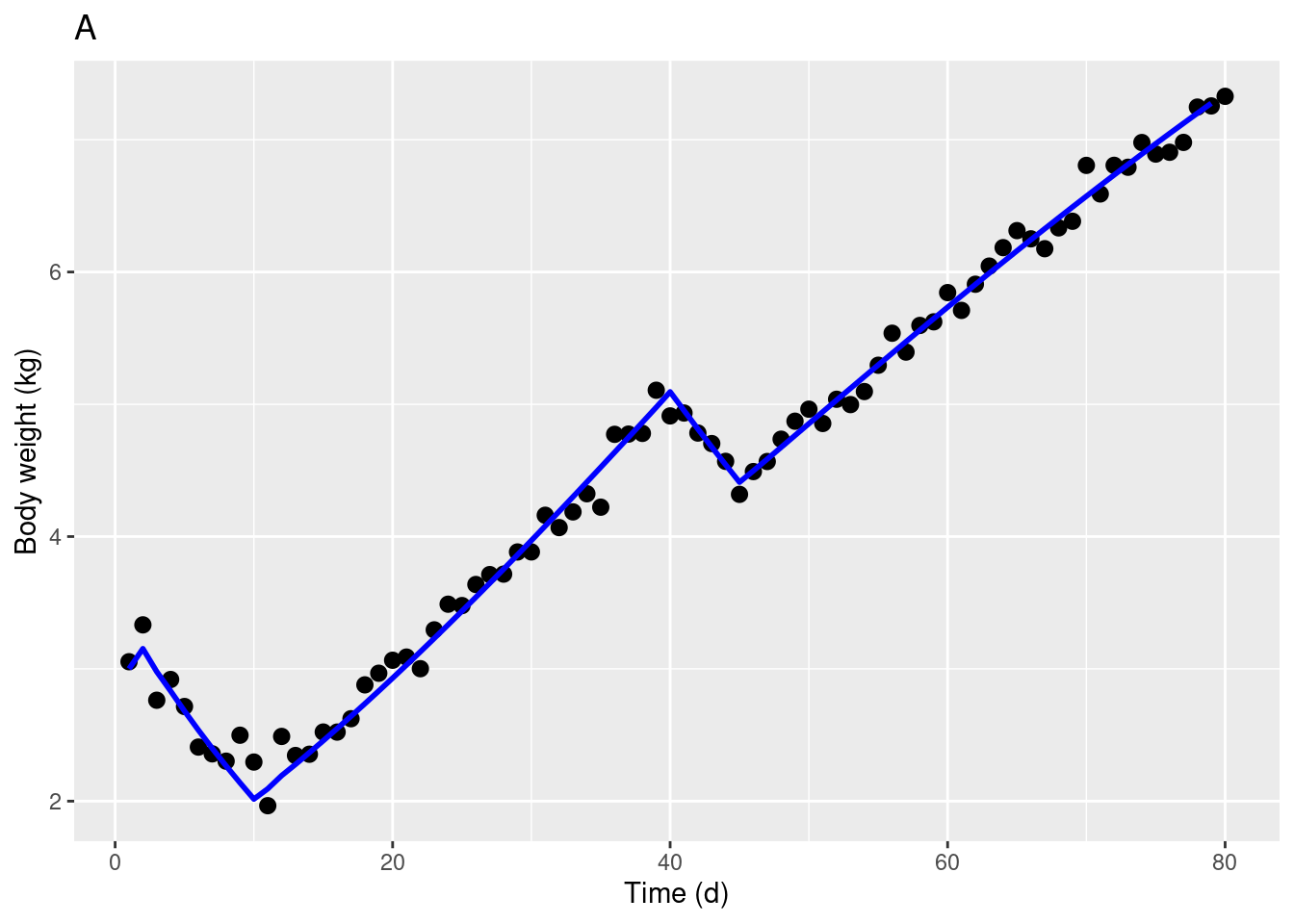

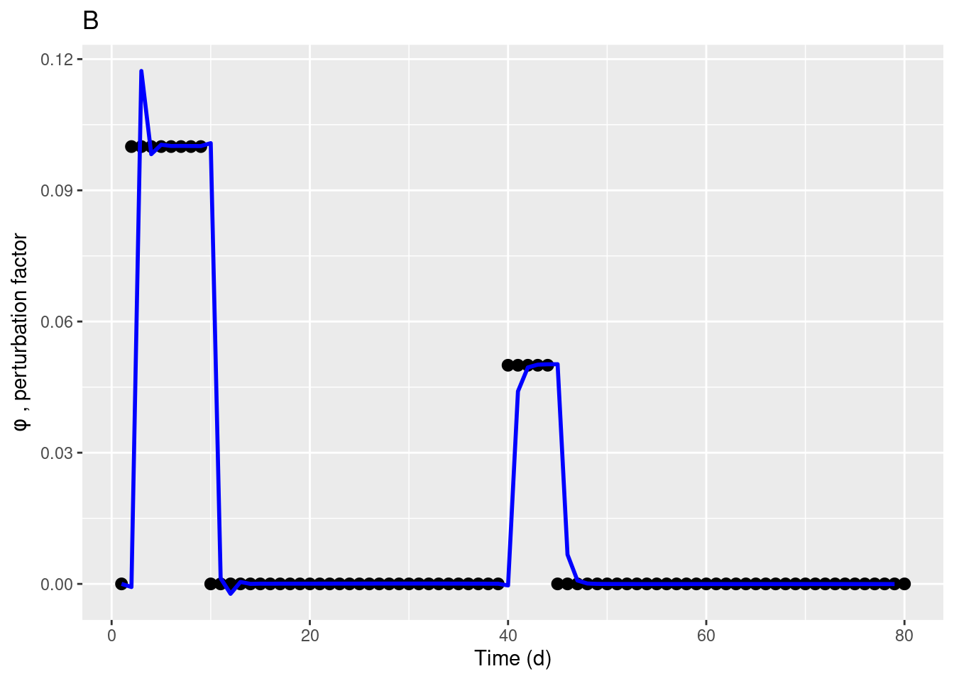
ggplot(DP, aes(tP, yP)) + geom_point(colour = 'black', size = 2.5)  + labs(title="B", x="Time (d)", y=expression(phi~ ", perturbation factor")) +
  geom_line(data = Dout, aes(tout,y2), size = 1, linetype = 1, colour = "blue" )

Warning: Removed 1 row containing missing values (`geom_line()`).